2 · Solve for coefficients

Chapter 1 left us with an impossible ask: find the function I(z) satisfying an integral equation at every point on the wire. Computers do neither of those things. The method of moments is the standard two-step retreat to something a computer can do:

Step 1 — expand. Stop looking for an arbitrary function. Write the current as a weighted sum of N fixed basis functions you chose in advance:

I(z) ≈ I₁·P₁(z) + I₂·P₂(z) + … + I_N·P_N(z)

The unknowns are now N numbers — the coefficients Iₙ — not a function.

Step 2 — test. You can’t enforce the boundary condition at every point with only N degrees of freedom, so enforce it N ways — one equation per segment. N equations, N unknowns:

Z · I = V

Z[m][n] = the field that basis function n produces at segment m — one integral you can compute numerically, since the basis function is a known shape. V[m] = the applied field at segment m. The physics is in filling Z; the answer is one call to a linear solver.

The simplest possible basis is the pulse: chop the wire into N segments; Pₙ(z) is 1 on segment n, 0 elsewhere. The current becomes a staircase.

The 2n+1-point grid

Here is the small idea that makes pulses actually work. Describe the wire’s n segments with 2n+1 points — the n+1 endpoints and the n midpoints:

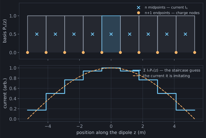
The midpoints carry the current — one pulse amplitude Iₙ each. The endpoints carry the charge. A wire holds charge wherever its current changes (ρ ∝ dI/dz, conservation of charge), and a staircase current changes exactly at the segment joints — so a pulse deposits a little pile of charge at each endpoint.

That split is the whole trick. The field of the wire has two parts: a vector-potential part driven by the current (the moving charge), and a scalar-potential part driven by the charge itself (the piles at the endpoints). Keep them separate — current at the midpoints, charge at the endpoints — and the naive scheme converges. (Skip the split, and matching a pulse current against the raw kernel from chapter 1 famously does not converge — a cautionary tale we’ll leave to the literature.)

The idea in forty lines

Pulses, the current/charge split, and the thin-wire kernel from chapter 1, verbatim from the primer’s own repo (site/figures/toy_solver.py):

import numpy as np

C0 = 299792458.0  # m/s
EPS0 = 8.8541878188e-12  # F/m
MU0 = 1.25663706127e-6  # H/m


def toy_dipole(L, a, wavelength, N):
    """Input impedance of a center-fed dipole: length L, wire radius a,
    N segments (odd, so one segment straddles the center), 1 V delta gap."""
    k = 2 * np.pi / wavelength
    omega = 2 * np.pi * C0 / wavelength
    dz = L / N

    # 2N+1 points: interleaved endpoints (even index) and midpoints (odd index).
    pts = np.linspace(-L / 2, L / 2, 2 * N + 1)
    mid = pts[1::2]  # N segment centers  — where the current lives
    lo, hi = pts[0:-1:2], pts[2::2]  # each segment's two endpoints — where charge sits

    def psi(A, B):
        """Green's-function kernel between every point in A and B, with the
        analytic self-term where two points coincide (the wire's own surface)."""
        R = np.abs(A[:, None] - B[None, :])
        same = R < dz / 1e6
        R[same] = 1.0  # avoid 0/0; overwritten below
        out = np.exp(-1j * k * R) / (4 * np.pi * R)
        out[same] = np.log(dz / a) / (2 * np.pi * dz) - 1j * k / (4 * np.pi)
        return out

    # Vector potential (from the current): both segments tested at their centers.
    Z = 1j * omega * MU0 * dz**2 * psi(mid, mid)
    # Scalar potential (from the charge): the endpoint charges of segment n,
    # differenced across the endpoints of segment m. This is the -∇φ term.
    Z += (psi(hi, hi) - psi(lo, hi) - psi(hi, lo) + psi(lo, lo)) / (1j * omega * EPS0)

    # Delta-gap feed: 1 V across the center segment.
    v = np.zeros(N, dtype=complex)
    v[N // 2] = 1.0
    I = np.linalg.solve(Z, v)
    return 1.0 / I[N // 2], I, mid  # Z_in = V / I(feed), with V = 1

That’s a complete method-of-moments solver, and it’s essentially Harrington’s classic straight-wire example (Harrington, Field Computation by Moment Methods, 1968). Two lines carry the physics. psi is the Green’s-function kernel — chapter 1’s a² floor, hidden here in the analytic self-term log(dz/a)/(2π dz) for the one integral that would otherwise divide by zero (source and observation on the same segment, the wire on top of itself). And the four-cornered difference psi(hi,hi) − psi(lo,hi) − psi(hi,lo) + psi(lo,lo) is the scalar potential: the segment’s two endpoint charges, differenced across the observation segment’s two endpoints. Everything else is the two-step retreat: np.linalg.solve is the whole “simultaneous everywhere” character of the problem collapsing into linear algebra.

The moment of truth

Run it on the real specimen — L = 10.582, a = 0.0005, λ = 22:

Z_in, I, z_mid = toy_dipole(10.582, 0.0005, 22.0, 161)
# Z_in ≈ 70.9 - 8.7j ohms

momwire’s B-spline solver says 69.6 − 18.3j (and, spoiler for chapter 7, an independent NEC-2 engine agrees). The toy’s resistance is already right to about a percent; its reactance is in the right neighbourhood and closing. This is a working solver, on the actual antenna — no fattened wire, no magic segment count. Its staircase current sits right on top of momwire’s smooth one:

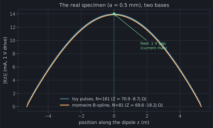
Both bases agree on the whole shape, right up to the current maximum at the feed (marked) — the 1 V delta gap where the generator sits. This is a near-half-wave dipole, so the current crests at the feed and tapers to zero at the tips: the same physical current, resolved two completely different ways. When the method works, it works. (It also, we’ll see in chapter 3, works slowly — but let’s enjoy the win first.)

What the matrix knows

Before moving on, look at the object the toy built. Here is log₁₀|Z[m][n]| for the specimen at N = 81:

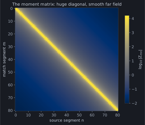
Two things to file away:

• The diagonal screams. Self- and neighbour-interactions (that sharp kernel peak from chapter 1, and the analytic self-term) tower over everything else. All the delicate integration happens within a few segments of the diagonal.
• Away from the diagonal, the matrix is smooth and boring. The field of segment 10 at segment 60 barely differs from its field at segment 61. Distant interactions carry almost no independent information — the matrix is, in a precise sense we’ll meet in Act IV, secretly low-rank. That boredom is worth a 12× speedup on real arrays; it is the entire business model of hmatrix and arrayblock.

What momwire does instead

The toy uses the crudest possible basis. momwire’s two dense solvers commit to better ones:

• SinusoidalSolver expands in NEC-2’s three-term basis — constant + sin(kz) + cos(kz) per segment — shapes that already look like solutions of the wave equation, so a handful of them fit a physical current superbly (chapter 4).
• BSplineSolver expands in degree-1/2 B-splines — smooth piecewise polynomials with guaranteed continuity, extending cleanly to bent wires and multi-wire junctions (chapter 5) — and replaces our blunt per-segment testing with Galerkin testing: demand the residual be orthogonal to every basis function, not merely balanced segment by segment.

Why bother, when the toy already works? Because “works” and “works cheaply” are different claims — and we quietly dodged both the question of how many segments that took and the meaning of the one line we typed without comment: the feed. Chapter 3 collects on both.