6 · Integrals done honestly
The sinusoid of chapter 4 filled two-thirds of its matrix for free, because the wave operator annihilated its sine and cosine pieces. The B-spline of chapter 5 has no such luck: a polynomial current is not a solution of the wave equation, so every matrix entry is a genuine integral of chapter 1’s kernel against two basis functions. Most are easy. A few will ruin your day. Telling them apart — and treating each honestly — is the unglamorous craft that decides whether the whole solver is accurate. As the saying in this field goes: MoM is 90% quadrature engineering.
Two neighbours, two integrands
Section titled “Two neighbours, two integrands”Filling entry Z[m][n] means integrating the kernel g(s, s′) = e^{−jkR}/(4πR)
as the source point s′ runs across segment n and the observation point sits
on segment m. Whether that integral is trivial or treacherous depends entirely
on how far apart the two segments are:
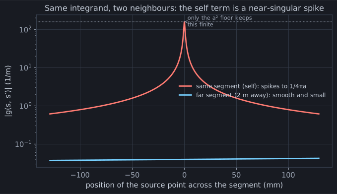
For a far pair, the integrand is a gently curved line — the kernel barely
changes as the source crawls across a distant segment. For the self pair
(and its close neighbours), the source point passes directly under the
observation point, R collapses toward the wire radius a, and the integrand
spikes to 1/4πa — here about 160, held finite only by chapter 1’s a²
floor. Same formula, wildly different shape, and Gauss-Legendre quadrature feels
the difference brutally.
You can’t out-integrate a singularity
Section titled “You can’t out-integrate a singularity”Point a fixed quadrature rule at both and watch:
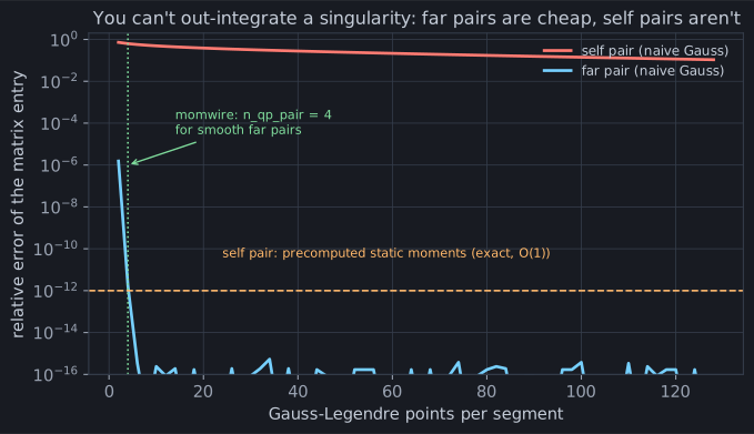
The far pair is nailed to machine precision by four points — the integrand is
smooth, and Gauss quadrature is exact for smooth things almost immediately. The
self pair is a disaster: at one hundred and thirty points it is still ~100%
wrong. The spike is half a millimetre wide sitting in a segment a quarter of a
metre long; the Gauss nodes step right over it, never seeing the thing that
carries most of the integral. Adding points barely helps — you would need nodes
spaced finer than a across the whole segment, thousands of them, and even then
you’d converge slowly. This is the same wall Act I’s pulse toy hit, and the same
lesson: you cannot out-integrate a singularity; you have to handle it.
The split
Section titled “The split”So momwire refuses to try. It splits the two cases and gives each what it needs
(BSplineSolver,
constructor knobs n_qp_pair and the static-moment path):
- Far and near-but-not-touching pairs get plain Gauss-Legendre with
n_qp_pair = 4nodes — from the memoized_quadrature.py(all thirty lines of it:leggaussis not free, so cache it). Four is plenty, and the solver won’t even let you go past eight — beyond that the smooth integrand has nothing left to give. - Self and edge-sharing pairs get the singular integral precomputed
analytically as static moments — the integral of the
1/Rsingularity against each pair of B-spline pieces, worked out once in closed form (scripts/derive_bspline_static_moments.py→ the big table in_bspline_static_moments.py). At runtime the treacherous entry is a table lookup, not an integral.
They’re called static moments for a reason worth its own sentence: the
singular geometry — how a 1/R behaves against two overlapping splines — does
not depend on frequency. So it’s computed once and reused at every
wavenumber. When chapter 3’s swept solver evaluated 46 frequencies in 65 ms,
this is why: the hard part of every matrix was already done, frequency-free.
Run it yourself
Section titled “Run it yourself”Because the smooth part is genuinely converged at four points and the singular
part isn’t integrated numerically at all, the n_qp_pair knob is nearly inert —
which is exactly the sign of a quadrature scheme that has nothing left to prove:
import numpy as npfrom momwire import BSplineSolver
wire = np.array([[0.0, -5.291, 0.0], [0.0, 5.291, 0.0]])for nq in (2, 4, 8):    Z, _ = BSplineSolver(wires=[wire], nsegs=21, wavelength=22.0, wire_radius=0.0005,                         degree=2, n_qp_pair=nq,                         feed_wire_index=0, feed_arclength=5.291).compute_impedance()    print(f"n_qp_pair={nq}:  {Z.real:.4f} {Z.imag:+.4f}j")# n_qp_pair=2:  69.6634 -18.3665j# n_qp_pair=4:  69.6635 -18.3652j# n_qp_pair=8:  69.6635 -18.3648j   — two-thousandths of an ohm across the range
The matrix is now filled honestly — smooth where it can be, exact where it must be. Which raises the question this whole act has been circling: filled honestly or not, how would you know the final answer is right? Chapter 7 is the cross-examination — convergence, the knee, and an independent engine.