5 · Splines and junctions

Chapter 4’s sinusoidal basis is close to perfect on a straight wire — and that straight is the catch. NEC’s gorgeous closed-form coefficients are derived for a segment whose neighbours continue in a line; the moment the wire bends, branches, or meets three others at a junction, that derivation turns into casework. momwire’s workhorse basis gives up a little of the sinusoid’s per-segment cleverness to buy one thing: it stays simple on any shape.

A ladder of smoothness

The idea is the plainest one in numerical analysis: on each segment, let the current be a polynomial of degree d, and stitch the pieces together with d-fold continuity. These are B-splines. Two rungs matter here, and it’s worth seeing them against Act I’s pulse:

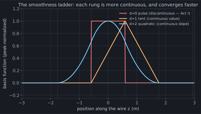
• d = 0 is the pulse — a box, discontinuous at every joint. Act I.
• d = 1 is the tent: piecewise linear, continuous in value. This is exactly the textbook “triangle” basis; momwire’s degree-1 B-spline is the tent, feed conventions aside.
• d = 2 is the quadratic: a smooth bell, continuous in value and slope.

Here is why that ladder is the same ladder from Act I, restated in the one quantity that matters. The charge is ρ ∝ dI/ds, and the scalar potential of that charge is where the reactance lives. So differentiate each rung:

• pulse → dI/ds is a train of delta functions (point charges — the knots that made Act I crawl);
• tent → dI/ds is piecewise constant (honest, distributed pulse charge);
• quadratic → dI/ds is itself continuous (the charge is now as smooth as the pulse’s current was).

Every rung up the smoothness ladder is a rung up the charge ladder — and the charge is what carries the reactance. That’s not a coincidence; it’s the whole story of Act I told in one derivative.

What the extra rung buys

On the specimen dipole, the convergence tracks the ladder exactly:

N	d=1 tent	d=2 quadratic
3	74.8 − 94.2j	69.9 − 18.1j
5	71.2 − 41.8j	69.8 − 18.5j
21	69.8 − 19.6j	69.7 − 18.4j

The quadratic is essentially converged at three segments — 69.9 − 18.1j against the true 69.6 − 18.3j — edging out even the sinusoid, because its charge is already smooth. The tent, one rung lower, needs a coarse handful more before its reactance settles. Same basis family, one parameter, and you dial accuracy against cost.

Junctions: where splines earn their keep

A real antenna is rarely one straight wire. It bends (an inverted-V), it branches (a top hat), it meets itself at nodes where three or more wires join. This is where the sinusoid’s closed forms give out and the spline just keeps working — because a junction is only a boundary condition, and a polynomial basis takes boundary conditions for breakfast.

The condition is Kirchhoff’s current law: the currents flowing into a junction node sum to zero. momwire enforces it as a constraint across the basis functions that touch the node — declare the node and the basis does the rest (BSplineSolver takes a junctions list of the wire-ends that meet). Here it is on a T — a downlead feeding two top arms:

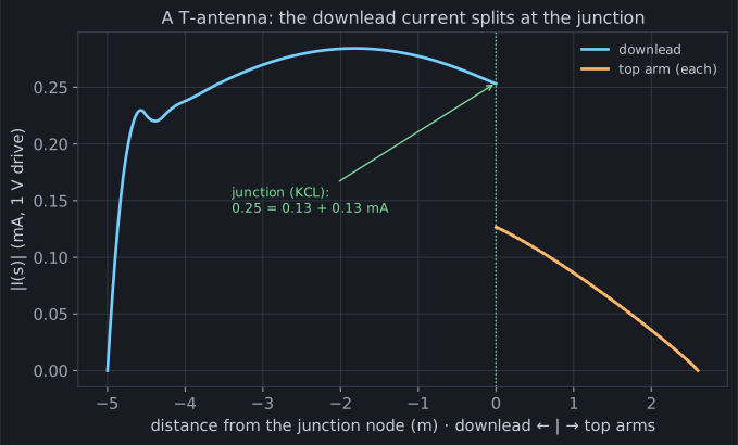
The downlead arrives at the node carrying 0.25 mA; it splits into the two top arms at 0.13 mA each. 0.25 = 0.13 + 0.13 — Kirchhoff, resolved by the basis, not by hand. Nothing about the solver changed from the straight dipole; we added two wires and named one node. That uniformity — one basis, any topology — is why momwire leans on B-splines for real antennas and keeps the sinusoid as a straight-wire cross-check.

Run it yourself

import numpy as np
from momwire import BSplineSolver

wire = np.array([[0.0, -5.291, 0.0], [0.0, 5.291, 0.0]])
solver = BSplineSolver(wires=[wire], nsegs=3, wavelength=22.0,
                       wire_radius=0.0005, degree=2,
                       feed_wire_index=0, feed_arclength=5.291)  # 1 V at the center
Z, coeffs = solver.compute_impedance()
print(f"d=2, N=3:  Z_in = {Z.real:.1f} {Z.imag:+.1f}j ohms")   # 69.9 -18.1j — three segments

Three quadratic segments, converged. But that innocent compute_impedance hides a debt the sinusoid didn’t owe: a polynomial current does not do its own quadrature. Every matrix entry is now a genuine integral of the kernel against a spline — and some of those integrals are nearly singular. Chapter 6 is about paying that debt honestly, because “MoM is 90% quadrature engineering.”

Turn the knob yourself

The antennaknobs simulator runs the B-spline engine on real, branched geometries — build an antenna that bends and watch the current stay continuous through every joint.